Introduction
How good is your prediction ŷ? If you are predicting the label y of a new object, how confident are you that y = ŷ? If the label y is a number, how close do you think it is to ŷ? In machine learning, these questions are usually answered in a fairly rough way from past experience. We expect new predictions to fare about as well as past predictions.
One of the disadvantages of machine learning as a discipline is the lack of reasonable confidence measure for any given prediction.
Conformal prediction uses past experience to determine precise levels of confidence in new predictions. Given an error probability ε, together with a method that makes a prediction ŷ of a label y, it produces a set of labels, typically containing ŷ, that also contains y with probability 1 − ε. Conformal prediction can be applied to any method for producing ŷ: a nearest-neighbor method, a support-vector machine, ridge regression, etc.
A short introduction to the main components of Conformal Prediction is outlined below. Interested readers may refer to a full treatment of Conformal Prediction in our book [1].
Nonconformity
Intuitively, nonconformity measure is a way of measuring how different a new example is from old examples. Formally, a nonconfomnity measure is a measurable mapping
$A : Z^{(*)} \times Z \rightarrow \overline{R}$
to each possible bag of old examples and each possible new example, A assigns a numerical score indicating how different the new example is from the old ones.
It is easy to invent nonconformity measures, especially when we already have methods for prediction at hand:
If the examples are merely numbers $(Z = R)$ and it is natural to take the average of the old examples as the simple predictor of the new example, then we might define the nonconformity of a new example as the absolute
value of its difference from the average of the old examples. Alternatively, we could use instead the absolute value of its difference from the median of the old examples.
In a regression problem where examples are pairs of numbers, say $z_i =(x_i, y_i)$, we might define the nonconformity of a new example $(x, y)$ as the absolute value of the difference between $y$ and the predicted value $\hat{y}$ calculated from $x$ and the old examples.
p-values
Given a nonconformity measure $(A_n)$ and a bag $\rmoustache z_1, \dots, z_n \lmoustache$, we can compute the nonconformity score
$\alpha_i := A_n(\rmoustache z_1, \dots, z_{i-1}, z_{i+1}, \dots, z_n \lmoustache, z_i)$
for each example $z_i$ in the bag. Because a nonconformity measure $(A_n)$ may be scaled however we like, the numerical value of $\alpha_i$ does not, by itself, tell
us how unusual $(A_n)$ finds $z_i$ to be. For that, we need a comparison of $\alpha_i$ to the other $\alpha_j$.
A convenient way of making this comparison is to compute the fraction
$\frac{|\{j=1, \dots, n : \alpha_j \geq \alpha_i\}|}{n}$
This fraction, which lies between $l/n$ and 1, is called the p-value for $z_i$. It is the fraction of the examples in the bag as nonconforming as $z_i$.
If it is small (close to its lower bound $1/n$ for a large n), then $z_i$ is very nonconforming (an outlier).
If it is large (close to its upper bound 1), then $z_i$ is very conforming
Conformal predictors
Every nonconformity measure determines a confidence predictor. Given a new object $x$, and a level of significance, this predictor provides a prediction set that should contain the object's label $y_n$.
We obtain the set by supposing that $y_n$, will have a value that makes $(x_n,y_n)$ conform with the previous examples.
The level of significance determines the amount of conformity (as measured by the p-value) that we require.
Formally, the conformal predictor determined by a nonconformity measure $(A_n)$ is the confidence predictor $\Gamma$ obtained by setting
$\Gamma^{\epsilon}(x_1, y_1, \dots, x_{n-1},y_{n-1},x_n)$
equal to the set of all labels $y \in Y$ such that
$\frac{|\{i=1,\dots,n:\alpha_i \geq \alpha_n\}|}{n} > \epsilon$
where
$\alpha_i := A_n(\rmoustache (x_1,y_1),\dots,(x_{i-1},y_{i-1}),(x_{i+1},y_{i+1}),\dots,(x_{n-1},y_{n-1}),(x_n,y)\lmoustache,(x_i,y_i)), i=1,\dots,n-1$
$\alpha_n := A_n(\rmoustache (x_1,y_1),\dots,(x_{n-1},y_{n-1})\lmoustache,(x_n,y))$
A tutorial
Applications
Conformal Prediction has been widely applied to many practical real life challenges. Below are some examples, extracted from our book [2].
Biometrics and Face Recognition
The challenge for face recognition comes from uncontrolled settings affecting image quality, and incomplete or deceiving information characteristic of occlusion and/or disguise.
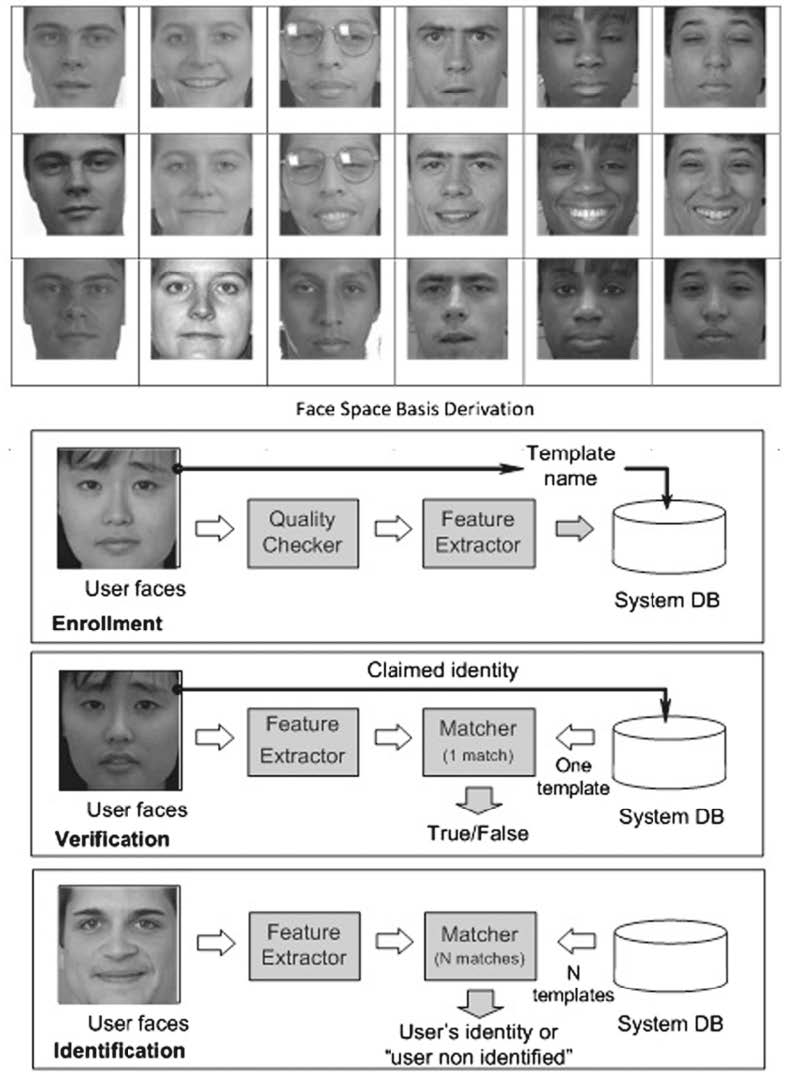
The nonconformity measure A used throughout is that of strangeness. The conformal predictor corresponding to A as a nonconformity measure employs p-values.
The particular strangeness and p-values used throughout are defined in the following
The strangeness measures the lack of typicality (for a face or face component) with respect to its true or putative (assumed) identity label and the labels for all the other faces or parts thereof known to some gallery G. Formally, the k-nn strangeness measure
$\alpha_i$ is the (likelihood) ratio of the sum of the k nearest neighbor (k-nn) distances d for sample xi from the same class y divided by the sum of the k nearest neighbor
(k-nn) distances from all the other classes (¬y). The smaller the strangeness, the larger its typicality and the more probable its (putative) label y is. We note here the impact
of nearest-neighborhood relations, characteristic of lazy learning, on the computation involved in the derivation of nonconformity measures (NCM).
An alternative definition for NCM as hypothesis margin, similar to the strangeness, is
$\Phi(x) = (||x - nearmiss(x)|| - ||x - nearhit(x)||) $
with nearhit (x) and nearmiss (x) being the nearest samples of x that carry the same and a different label, respectively. The strangeness can also be defined using the
Lagrange multipliers associated with (kernel) SVM classifiers but this requires a significant increase in computation.

Biomedical Diagnostic and Prognostic
There are several important advantages in applying conformal predictors (CP) in medical diagnostics. First of all, CPs provide valid measures of confidence in the
diagnosis, and this is often a crucial advantage for medical decision-making since it allows the estimation of risk of an erroneous clinical decision for an individual
patient. Moreover, the risk of clinical errors may be controlled by an acceptable level of confidence for a given clinical decision and therefore the risk of misdiagnosis is
known.Another feature that makesCPs an attractivemethod in medical applications is that they are region predictors. This means that if we do not have enough information
to make a definitive diagnosis, the method would allow us to make a number of possible (multiple) diagnoses and a patient may require further tests to narrow down the available options.
An example of conformal methods applied to proteomic (breast cancer diagnosis) was a part of blind comparative assessment organized by Leiden University Hospital.
The conformal predictor approach in this competition performed very well. Data from 117 patients and 116 healthy volunteers were obtained. The data were divided into a calibration (or training) set and a validation (or testing) set.
The training set consisted of 153 samples, 76 of which were cases and 77 controls. The test set consisted of 78 samples, 39 of which were cases (class 1) and 39 controls (class 2).
One potential complicating is that the data for the training set were obtained from two plates, and the data for the test set were taken from a third plate. Since the mass spectrometer is recalibrated prior to the analysis of each plate, there is a potential for differences between the training and testing sets to be introduced.
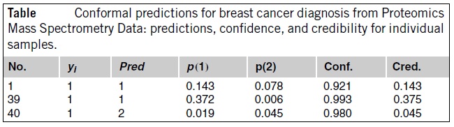
The table below shows several individual examples with confident predictions. The first column is ID number, the second one is the true diagnosis (1 for cases and 2 for the controls), the third is the forced prediction, the fourth and fifth columns are p-values for the corresponding hypotheses, and the sixth and seventh are confidence and credibility.
To interpret the numbers in Table 11.1, recall that high (i.e., close to 100%) confidence means that we predicted a diagnosis and the alternative diagnosis is unlikely.
If, say, the first example (No. 1) were classified wrongly, this would mean that a rare event (of probability less than 8%) had occurred; therefore, we expect the prediction to be correct (which it is).
For the diagnostic tasks using functional MRI (fMRI), there were 19 cases of depression and 19 controls. The attributes are 197484 MRI voxels (volume 2 × 2 × 2 mmpixels of the three-dimensional map), each of them measuring a blood oxygenation
signal that changes relative to baseline (crosshair fixation) during the observation of stimulus (standardized face expressing increasing levels of sadness).
For prognoses in depression, structured MRI (sMRI)was used. The datawere split into two classes of size 9 according to their reaction to a treatment: depressed subjects
who responded to an antidepressant treatment (class 1) and class 2 of nonresponders. The patients were examined by structural MRI scans while they were in an acute
depressive episode, prior to the initiation of any treatment, and clinical response was assessed prospectively following eight weeks of treatment with an antidepressant medication.
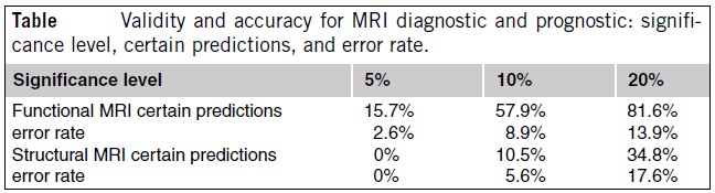
The overall results are presented in the table below. The validity property is demonstrated, in that prediction error rate is bounded by the significance level. Also, increasing
the significance level results in an increase in the number of certain predictions. For example, for the structural MRI dataset at the 5% significance level the algorithm
could not produce any definitive prognoses. Such result is due to the small sample sizes of this dataset.
Network Traffic Classification and Demand Prediction
One of the key requirements for dynamic resource allocation framework is to predict traffic in the next control time interval based on historical data and onlinemeasurements of traffic characteristics over
appropriate timescales. Predictions with reliability measures allow service providers and network carriers to effectively perform a cost-benefit evaluation of alternative
actions and optimize network performance such as delay and information loss.
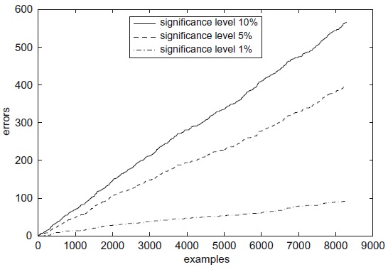
We extend conformal predictors to the case of time series. To do this, however, we have to either violate or change the restriction on the data required by the algorithm.
Thus, we lose the guarantee of validity given by conformal predictors. However, our experiments show that the error rate line is close to a straight line with the slope equal to the significance level (a parameter of the algorithm), which indicates empirical validity.
One way of using conformal predictors for time series data is to assume that there is no long-range dependence between the observations. In this scenario, we use a parameter $T \in N$, which specifies how many of the previous observations the current observation can depend on.
Suppose we have time series data $a1, a2, a3, \dots$ where $a_i \in R \forall i$. We employ two methods to generate pairs (object, label) from the time series data. If we want to generate as many pairs as possible and at the same time we do not mind violating the
exchangeability requirement, we use the rule
$\forall i, T+1 \leq i \leq n : z_i=(x_i,y_i) := ((a_{i-T}, \dots, a_{i-1}),a_i)$
where n is the length of the time series data. We call these observations dependent. If, on the other hand, we want to achieve validity, then we use the rule
$\forall 0 \leq i \leq [\frac{n}{T+1}] - 1 : z_i = (x_i,y_i) := ((a_{n-i(T+1)-T}, \dots, a_{n-i(T+1)-1}),a_{n-i(T+1)}) $
where $[k]$ is the integer part of k. These observations are called independent.
 [1] Algorithmic Learning in a Random World

Summary
Algorithmic Learning in a Random World describes recent theoretical and experimental developments in building computable approximations to Kolmogorov's algorithmic notion of randomness.
Based on these approximations, a new set of machine learning algorithms have been developed that can be used to make predictions and to estimate their confidence and credibility in high-dimensional spaces under the usual assumption that the data are independent and identically distributed (assumption of randomness). Another aim of this unique monograph is to outline some limits of predictions: The approach based on algorithmic theory of randomness allows for the proof of impossibility of prediction in certain situations. The book describes how several important machine learning problems, such as density estimation in high-dimensional spaces, cannot be solved if the only assumption is randomness.
 [2] Conformal Prediction for Reliable Machine Learning: Theory, Adaptations and Applications

Summary
The conformal predictions framework is a recent development in machine learning that can associate a reliable measure of confidence with a prediction in any real-world pattern recognition application, including risk-sensitive applications such as medical diagnosis, face recognition, and financial risk prediction.
Conformal Predictions for Reliable Machine Learning: Theory, Adaptations and Applications captures the basic theory of the framework, demonstrates how to apply it to real-world problems, and presents several adaptations, including active learning, change detection, and anomaly detection. As practitioners and researchers around the world apply and adapt the framework, this edited volume brings together these bodies of work, providing a springboard for further research as well as a handbook for application in real-world problems.
[3] A tutorial on conformal prediction
Abstract
Conformal prediction uses past experience to determine precise levels of confidence in new predictions. Given an error probability ε, together with a method that makes a prediction ŷ of a label y, it produces a set of labels, typically containing ŷ, that also contains y with probability 1 – ε. Conformal prediction can be applied to any method for producing ŷ: a nearest-neighbor method, a support-vector machine, ridge regression, etc.
Conformal prediction is designed for an on-line setting in which labels are predicted successively, each one being revealed before the next is predicted. The most novel and valuable feature of conformal prediction is that if the successive examples are sampled independently from the same distribution, then the successive predictions will be right 1 – ε of the time, even though they are based on an accumulating data set rather than on independent data sets.
In addition to the model under which successive examples are sampled independently, other on-line compression models can also use conformal prediction. The widely used Gaussian linear model is one of these.
[4] Conformal prediction with neural networks
Abstract
Conformal prediction (CP) is a method that can be used for complementing the bare predictions produced by any traditional machine learning algorithm with measures of confidence. CP gives good accuracy and confidence values, but unfortunately it is quite computationally inefficient. This computational inefficiency problem becomes huge when CP is coupled with a method that requires long training times, such as neural networks.
In this paper we use a modification of the original CP method, called inductive conformal prediction (ICP), which allows us to a neural network confidence predictor without the massive computational overhead of CP The method we propose accompanies its predictions with confidence measures that are useful in practice, while still preserving the computational efficiency of its underlying neural network.
[5] Criteria of efficiency for conformal prediction
Abstract
We study optimal conformity measures for various criteria of efficiency in an idealised setting. This leads to an important class of criteria of efficiency that we call probabilistic; it turns out that the most standard criteria of efficiency used in literature on conformal prediction are not probabilistic.